Tutorial on the usage of SCP tool

Here two examples on how to use the SCP class for different polymers will be illustrated.

Before starting any analysis, load the neccesary modules for this class.

from  utils_mda import MDA_input
#from pysoftk.pol_analysis.tools.utils_mda import MDA_input
from utils_tools import *
#from pysoftk.pol_analysis.tools.utils_tools import *
from clustering import SCP
#from pysoftk.pol_analysis.clustering import SCP


import numpy as np
import pandas as pd

Branched topology example

Select your trajectory files, it is recommended to use a tpr file for the topology and xtc file for the trajectory. Note that any MDAnalysis supported file can be used here.

topology='data/short_movie_branched.tpr'
trajectory='data/short_movie_branched.xtc'

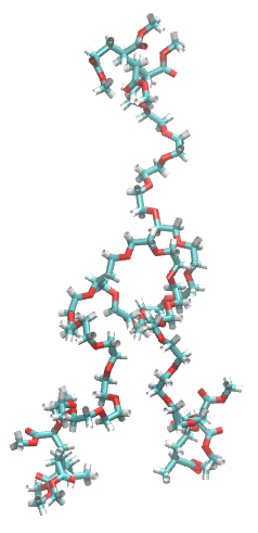
This is how the branched polymer looks:

We need to select the atoms on which the clustering will be applied. In this case this branched polymer has the hydrophobic block at the end of each arm. Since this polymer is amphiphilic and it is simulated in a box with water, it will form micelles. This micelle will be driving by the hydrophobic effect, meaning that polymers will be interacting via their hydrophobic blocks (to form the micelle). Therefore, the atoms that we decide to choose are the atoms in the middle of each hydrophobic block (so 3 atoms, 1 per arm).

atom_names = ['C02B', 'C01K', 'C02N']

We need to define the cluster cutoff. This will be the value use to determine if two polymers are part of the same micelle. Selecting this value may be an iterative process, but we suggest to use values ranging from 10 to 12 Å. But again, this will depend on the system being simulated.

cluster_cutoff = 12

Finally, before running the SCP tool, we need define the output path. Also, we need to define the start frame, stop frame and step between frames that we want to run the analysis on.

results_name='data/pictures_tutorial/branched_scp_result'
start=0
stop=10001
step=1

Now we are ready to run the SCP tool!

c = SCP(topology, trajectory).spatial_clustering_run(start, stop, step, atom_names, cluster_cutoff, results_name)

100%|████████████████████████████████████████████████████████████████████████████████████████████████████████████████████████████████████████████| 3/3 [00:00<00:00,  9.86it/s]

The file data/pictures_tutorial/branched_scp_result.parquet has been successfully created.
Function spatial_clustering_run Took 1.5952 seconds

To visualize the result we can load the parquet file in this way:

df_results = 'data/pictures_tutorial/branched_scp_result.parquet'
df = pd.read_parquet(df_results)
df

	time	micelle_resids	micelle_size
0	0.0	[[1, 2, 3, 4, 5, 6, 7, 8, 9, 10, 11, 12, 13, 1...	[20]
1	500000.0	[[1, 2, 3, 4, 5, 6, 7, 8, 9, 10, 11, 12, 13, 1...	[20]
2	1000000.0	[[1, 2, 3, 4, 5, 6, 7, 8, 9, 10, 12, 15, 17, 1...	[16, 1, 1, 1, 1]

Cyclic topology example

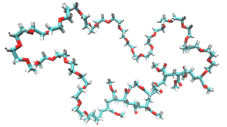
This is how the cyclic polymer looks:

We can follow the same steps applied on the branched example

topology='data/short_movie_cyclic.tpr'
trajectory='data/short_movie_cyclic.xtc'

results_name='data/pictures_tutorial/cyclic_scp_result'

cluster_cutoff = 12

start=0
stop=10001
step=1

However, since the topology is different, the atom selection will be different to the branched example, even though they are made from the same atoms. Since the polymer has a ring structure, we can just select the central atom of the hydrophobic block, as this is the only part of the polymer that will be interacting closely with the other hydrphobic blocks.

atom_names=['C02T']

Now, we can run the SCP tool

c = SCP(topology, trajectory).spatial_clustering_run(start, stop, step, atom_names, cluster_cutoff, results_name)

100%|███████████████████████████████████████████████████████████████████████████████████████████████████████████████████████████████████████████| 3/3 [00:00<00:00, 141.75it/s]

The file data/pictures_tutorial/cyclic_scp_result.parquet has been successfully created.
Function spatial_clustering_run Took 0.1356 seconds

To visualize the output

df_results = 'data/pictures_tutorial/cyclic_scp_result.parquet'
df = pd.read_parquet(df_results)
df

	time	micelle_resids	micelle_size
0	0.0	[[1, 2, 3, 4, 6, 7, 8, 11, 12, 13, 14, 15, 17,...	[15, 4, 1]
1	500000.0	[[1, 3, 12], [2, 4, 6, 7, 13, 14, 15, 17, 18, ...	[3, 11, 5, 1]
2	1000000.0	[[1, 3, 5, 8, 10, 12, 16], [2, 4, 6, 7, 13, 14...	[7, 11, 1, 1]