Modelling soft-matter long chain polymers

The PySoftK function pysoftk.topologies.diblock has been developed to address the challenge of creating patterned polymers. In this new version of PySoftK, we have enhanced the capabilities of this function for modelling long polymers. This tutorial explains how to use this function

Modelling long chains

PySoftK enables the use of xtb as a calculator employing a customized Force Field implementation (called xtb_ff). To introduce this functionality, one needs to import the corresponding RDKit auxiliary functions (line 1-2) and the needed modules from PySoftK as shown in the following snipet:

from rdkit import Chem
from rdkit.Chem import AllChem
from rdkit.Chem import rdDistGeom

from pysoftk.topologies.diblock import *
from pysoftk.format_printers.format_mol import *

To demonstrate the functionality of this module, two aminoacids (PEG and PGLA) are used to create a patterned-polymer (and stored in the variable mols). The pattern can be created in python-lists containing user-defined sequences of letters. In this case we have used 45 A’s and 15 B’s. This is displayed in the following snipet:

mols=[Chem.MolFromMolFile('peg.mol',removeHs=False), Chem.MolFromMolFile("pgla2.mol",removeHs=False)]

l1 = ["".join(["A" for i in range(45)])]
l2 = ["".join(["B" for i in range(10)])]

The script combines these lists and flattens them to create a single string (pattern) representing the entire block copolymer sequence as shown below:

pattern = "".join([item for sublist in [l1, l2] for item in sublist])

The Pt function from PySoftK takes the pattern string (pattern), loaded molecules (mols), a placeholder atom (“Br”). The key parameters of this function includes the relax_iterations (Number of relaxation steps for energy minimization), force_field (Force field used for energy calculations), swap_H (allow hydrogen swapping during block placement) and rot_steps (number of conformers during placement). This is observed in the following snippet:

a=Sm(mol_1,mol_2,"Br")
k=a.mon_to_poly()
new=Lp(k,"Br",4,shift=1.25).linear_polymer(250)

As shown in the previous example, the result of this operation is then printed in a PDB file called test.pdb, using the function FMT(object)pdb_print(name_to_be_printed).

new=Lp(k,"Br",4,shift=1.25).linear_polymer(250)
Fmt(new).xyz_print("test_2.xyz")

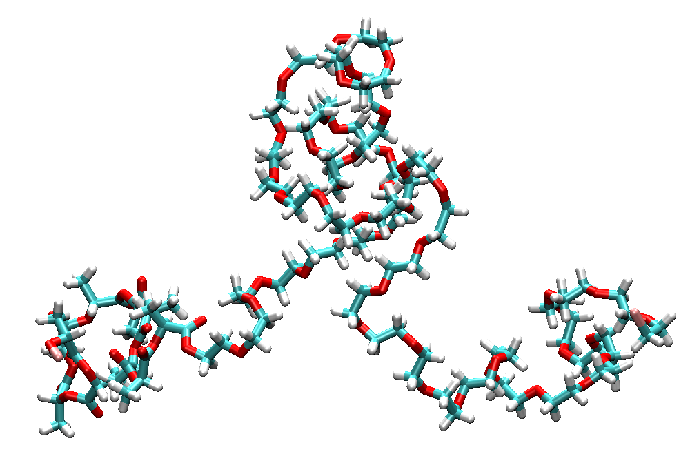
The results of the geometrical optimization are printed to the file test.pdb and can be visualized using VMD.